Tutorial for R users

In this tutorial we will enrich Acropora digitifera observations with bathymetry information. Please make sure you already followed the installation instructions.

We will first load the occurence file and create an enrichment file. As we download environment data, necessary metadata will be saved into that file.

Afterwards, we will pick a variable id from the catalog, and start downloading bathymetry data.

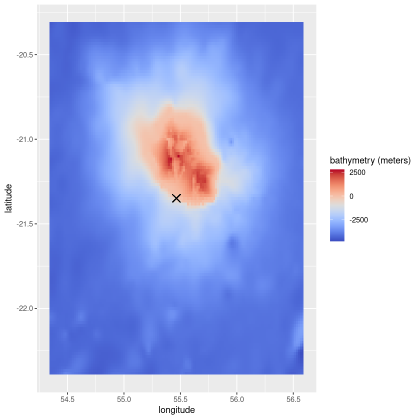
Finally, we will visualize the result for one of the occurrences.

[1]:

library(reticulate)

Load your occurrence data

[2]:

os <- import("os")
dataloader <- import("geoenrich.dataloader", convert=FALSE)
enrichment <- import("geoenrich.enrichment", convert=FALSE)

If you are using your own dataset (DarwinCore format)

A DarwinCore archive is bundled into the package for user testing (GBIF Occurrence Download 10.15468/dl.megb8n).

If you don’t have a dataset and you don’t want to register to GBIF yet you can use this one.

[3]:

example_path <- paste( os$path$split(dataloader$'__file__')[[1]],
                      '/data/AcDigitifera.zip', sep = '')
geodf <- dataloader$open_dwca(path = example_path)

If you are using your own dataset (csv format)

Fill in the path to your csv and the compulsory column names.

Additional arguments are passed down to pandas.read_csv

[ ]:

geodf <- dataloader$import_occurrences_csv(path = '', id_col = '', date_col = '', lat_col = '', lon_col = '')

If you do not have occurrences but want to enrich arbitrary areas

See documentation for information about input file format.

[4]:

example_path <- paste( os$path$split(dataloader$'__file__')[[1]] ,
                      '/data/areas.csv', sep = '')
df <- dataloader$load_areas_file(example_path)

Create enrichment file

[5]:

# For occurrences
dataset_ref_occ <- 'ac_digitifera'
enrichment$create_enrichment_file(geodf, dataset_ref_occ)

[ ]:

# For areas
dataset_ref_areas <- 'arbitrary_areas'
enrichment$create_enrichment_file(df, dataset_ref_areas)

Enrich

Define enrichment scope

We use the dataset reference that was used to create the enrichment file.

geo_buff is the buffer around the occurences (in kilometers).

time_buff specifies a temporal buffer. In this case we download data from 7 days before the occurrence date, to the occurrence date. time_buff is only used for variables that have a time dimension

[6]:

var_id <- 'bathymetry'
dataset_ref_occ <- 'ac_digitifera'
geo_buff <- 115
time_buff <- c(-7L, 0L)

Only enrich a small slice first to check speed.

[7]:

enrichment$enrich(dataset_ref_occ, var_id, geo_buff,
                  time_buff, slice = c(0L,100L))

For large areas, use downsample argument to download only part of available data (to reduce download time)

[ ]:

# Skip 9 latitude and longitude points for every downloaded point.
dataset_ref_areas <- 'arbitrary_areas'
downsample <- list('latitude'= 9L, 'longitude'= 9L)

enrichment$enrich(dataset_ref_areas, var_id, downsample = downsample)

Data retrieval

[8]:

exports <- import("geoenrich.exports")
enrichment <- import("geoenrich.enrichment", convert = FALSE)
dataset_ref <- 'ac_digitifera'
var_id <- 'bathymetry'

Check the enrichment status of the dataset.

[ ]:

enrichment$enrichment_status(dataset_ref)

Export summary statistics to a csv file

[9]:

exports$produce_stats(dataset_ref, var_id, out_path = './')

Export data as a raster layer for the first occurrence of the dataset

[ ]:

ids <- py_to_r(enrichment$read_ids(dataset_ref))
occ_id <- ids[[1]]

[ ]:

exports$export_raster(dataset_ref, occ_id, var_id, path = './')

Export data as a png file for the first occurrence of the dataset

[10]:

ids <- py_to_r(enrichment$read_ids(dataset_ref))
occ_id <- ids[[1]]

[11]:

exports$export_png(dataset_ref, occ_id, var_id, path = './')

Retrieve the raw data and plot it

Required libraries: ggplot2, reshape2, wellknown, pals

[12]:

library(ggplot2)
library(reshape2)
library(wellknown)
library(pals)

[13]:

output <- exports$retrieve_data(dataset_ref, occ_id, var_id, shape = 'buffer')

data <- output$values
unit <- output$unit
coords <- output$coords

# Retrieve coordinates
for (c in coords){
    if (c[[1]] == 'latitude'){
        lats = c[[2]]}
    if (c[[1]] == 'longitude'){
        longs = c[[2]]}}

# Retrieve coordinates of the occurrence
occurrences <- read.csv(file = paste(enrichment$biodiv_path, dataset_ref,  '.csv', sep = ''), row.names = 1)
occ_point <- wkt2geojson(occurrences[as.character(occ_id),]$geometry)$geometry$coordinates

[15]:

colnames(data) <- longs
rownames(data) <- lats
data_df <- melt(data)
colnames(data_df) <- c('latitude', 'longitude', var_id)
title <- paste(var_id, ' (', unit, ')', sep = '')
ggplot(data = data_df, aes(x=longitude, y=latitude, fill=eval(as.name(var_id)))) +
       geom_tile()+
       scale_fill_gradientn(title,colours=coolwarm(100), guide = "colourbar")+
       geom_point(aes(x=occ_point[[1]], y=occ_point[[2]]), shape=4, size = 4)